Anatomical Variation in the Knee: A Dataset of 3D Bone Models and Statistical Shape Models

Data Description

This dataset includes data and metadata for 102 subjects, 50 female and 52 male, from Asian (A, n = 12), Non-Hispanic Black or African American (NHB, n = 23), Hispanic (H, n = 21), Native American (NA, n = 24), and Non-Hispanic White (NHW, n = 22) racial or ethnic backgrounds sourced from the New Mexico Decedent Image Database (NMDID)¹. It includes raw and smoothed 3D models of the distal femur, proximal tibia, and distal fibula, along with corresponding segmentation masks derived from the source CT scans. Each subject is identified by a unique six-digit NMDID code, enabling association with the original scan data. Access to the NMDID requires completion of the database’s data access, sharing, and usage agreement. The dataset also contains registered instances of the distal femur and proximal tibia, in which subject-specific anatomies were represented using a common mesh topology and coordinate system. For the registered instances, correspondence was established by morphing a template mesh for an average-sized geometry to each anatomy in the training set using rigid and non-rigid registration methods. An SSM was developed from each register by applying principal component analysis to the registered nodal coordinates for each bone, the outcomes of which can be found in the associated manuscript. Metadata and selected morphological parameters are provided for each subject to facilitate characterization of anatomical variation.

Support

The creation of this data was supported in part by the University of Denver.
The original NMDID data (https://nmdid.unm.edu/) was made possible by the Free Access Decedent Database funded by the National Institute of Justice grant number 2016-DN-BX-0144.

Methods
Data Sourcing

Images were obtained from the New Mexico Decedent Image Database (NMDID), a comprehensive dataset containing whole-body CT scans and associated metadata for over 15,000 individuals who died in New Mexico between 2010 and 2017¹. Instances selected from the NMDID were curated to approximate the demographic composition of the United States population², as permitted by the NMDID data. Subjects were included if they were between 25 and 80 years of age and had a BMI of less than 40, based on cadaver height and weight. Exclusion criteria included a recorded history of cancers, tumors, or malignancies, documented lower limb injuries, a manner of death that could have resulted in lower limb injuries (e.g. motor vehicle accident), moderate or severe cadaver decomposition, or severe osteoarthritis.

Data Processing

Imaging data for each subject file downloaded from the NMDID database was comprised of 26 CT scans. The “thin bone torso” and “thin bone lower extremity” scans were used in this work. Before processing, a preliminary assessment of each subject's respective scans was conducted to check for factors that may render the subject unsuitable for modeling purposes, including the presence of moderate to severe osteoarthritis in the knee joints, intraosseous cannulae, orthopedic implants, scan artifacts within regions of interest, or movement artifacts between the torso and lower extremity scans. Both of the subject’s lower extremities were considered for use, with one leg ultimately included per subject. Left-sided anatomy was mirrored to the right. If neither leg proved appropriate for use, the subject was subsequently excluded from further analysis.

The subject's bony geometry was segmented from the "thin bone torso" (proximal femur) and "thin bone lower extremity" (distal femur, tibia, distal fibula) scans using ScanIP software (Synopsys, Mountain View, CA). To do this, image intensity thresholds were first adjusted to isolate bony tissue. The relevant anatomy (femur, tibia, and distal fibula) was separated from the resulting mask, and artifacts were removed using the “island removal” function. Working one bone at a time, gaps were corrected using the “close” and “gap filling” tools. Each slice was reviewed to ensure segmentation accuracy, with additional manual edits applied as necessary. The cavities in the mask were then filled, and smoothed masks were generated for each bone. Final masks were visually inspected for artifacts before being exported from ScanIP as STL files containing the surface geometry information for each bone. As the femur spanned the “thin bone torso” and “thin bone lower extremity” scans, it was saved as separate proximal and distal STL files.

STL files for each tibia and femur were imported into Hypermesh (Altair, Troy, MI). An anatomical coordinate system was established for each bone based on landmarks manually identified within the software. For the tibia, five bony landmarks were identified. The medial and lateral plateau centers were defined as the midpoints between the medial-anterior (1) and medial-posterior (2) plateau edges, and between the lateral-anterior (3) and lateral-posterior (4) plateau edges, respectively. The origin was defined as the midpoint between the two centers. The superior-inferior (SI, z) axis was defined from the ankle joint center (5), estimated as the midpoint between the medial and lateral malleoli, to the tibial origin, pointed superiorly. The anteroposterior (AP, y) axis was obtained by crossing the SI axis and the vector from the medial to lateral tibial plateau center, pointed anteriorly. The mediolateral (ML, x) axis was derived by crossing the SI and AP axes and was pointed laterally.

For the femur, an anatomical coordinate system was defined using three manually extracted bony landmarks: the hip joint center (1), approximated as the center of a best-fit sphere fit to three points on the femoral head surface, the medial epicondyle (2), and the lateral epicondyle (3). The origin was defined as the midpoint between the medial and lateral epicondyles. The superior-inferior (SI, z) axis was defined as the vector passing through the origin and hip joint center, pointed superiorly. The anteroposterior (AP, y) axis was obtained by crossing the SI axis and the vector from the medial to the lateral epicondyle, pointed anteriorly. As with the tibia, the mediolateral (ML, x) axis was derived by crossing the SI and AP axes and was pointed laterally.

The surface geometry of each tibia and femur, along with the corresponding landmarks, was then transformed from the global CT coordinate system into its respective anatomical coordinate system. The transformation matrices defining the relationship between the CT and anatomical coordinate systems were retained for future use.

Shape Modeling Workflow

Template geometries used were obtained from work previously done by Fugit et al³. In this work, an average-sized right tibia and femur were selected as the templates and aligned in their local coordinate systems as described above. A template mesh was constructed for tibial surfaces (20,296 nodes and 40,588 triangular elements, 0.95 ± 0.16 mm edge length) and femoral surfaces (49,767 nodes and 99,530 triangular elements, 0.82 ± 0.19 mm edge length). The diaphyses of the tibial and femoral template geometries were resected at a ratio of 1.38 and 1.74, respectively, between SI length and ML condylar width, retaining the distal femur and proximal tibia26.

Registration of the instances was fully automated in a MATLAB (MathWorks, Natick, MA) script, employing separate scripts for tibias and femur. The shafts of the instances were first resected per the template aspect ratio. An Iterative Closest Point-based algorithm⁴ was then used to rigidly align the instance to the template and then to affinely deform the template onto the instance. A Coherent Point Drift (CPD)-based algorithm completed the morphing of the template onto the instance⁵, with nodal coordinates of the final deformed template mesh recorded as the registered instance triangular mesh. Morphing error was quantified as the root mean square (RMS) error of the distances between the deformed template points and their respective closest point in the instance mesh. Additionally, element skewness and aspect ratio were computed for the elements of each registered mesh to monitor mesh quality. Skewness measures how close a triangular element is to ideal (equilateral), ranging from 0 (perfect) to 1 (degenerate)⁶. Aspect ratio compares the height and width of each triangle, with 1 representing a perfect element and higher values indicating increasing deviation from ideal⁶.

SSM Generation and Assessment

To ensure a consistent spatial alignment, all registered instances were rigidly aligned to the smallest specimen in each dataset using ICP. SSMs of the proximal tibia and distal femur were generated by performing principal component analysis on the final aligned registers. Morphological parameters for each tibia and femur instance were calculated using fully automated, previously developed MATLAB codes based on work from Mahfouz et al.⁷, Ma et al.⁸, Wang et al.⁹, and Van Oevelen et al¹⁰. To better understand the variation captured by each SSM, selected principal components (PCs) were visualized and correlated with the morphological parameters. Finally, model quality was evaluated by computing metrics of accuracy, compactness, generalizability, and specificity across various levels of PC inclusion¹¹.

Data Records

The dataset includes data and metadata for 102 subjects, 50 female and 52 male, with an average age of 45.3 (+/- 14.1) and 43.9 (+/- 13.9) years, respectively. Subjects came from Asian (A, n = 12), Non-Hispanic Black or African American (NHB, n = 23), Hispanic (H, n = 21), Native American (NA, n = 24), and Non-Hispanic White (NHW, n = 22) racial or ethnic backgrounds. NMDID race and ethnicity metrics were self-reported by the decedents in the 2010 census. Please note that for the purposes of this work, "Hispanic" refers to decedents who identified as racially Hispanic, reflecting the usage in the 2010 census where many New Mexicans selected Hispanic as an "Other" race option.

Each subject is identified by a unique six-digit NMDID code, enabling association with the original scan data. Access to the NMDID requires completion of the database’s data access, sharing, and usage agreement. For each subject, the dataset includes select metadata and morphologic parameters, raw and smoothed segmentation masks for the tibia, femur, and fibula of a single lower extremity; raw and smoothed segmented bony anatomy in CT space; and registered bony anatomy for the distal femur and proximal tibia.

• • Metadata:
  • Metadata are provided in the Excel file Metadata_and_MorphologicalParameters.xlsx under the ‘Metadata’ worksheet and are organized by NMDID identifier. The included data fields are sex, age (years), race, ethnicity, additional ancestry information, socioeconomic status (childhood), socioeconomic status (adulthood), living height (cm), living weight (kg), cadaver height (cm), BMI, and laterality of the segmented limb (left or right). Information on metadata collection protocols and metadata may be obtained through the NMDID.
• • Morphological parameters:
  • Calculated morphological parameters are provided in the same Excel file under the ‘Morphological Parameters’ worksheets and are organized by NMDID identifier. These parameters are also available in MATLAB within the Registers.mat structure under the field MP. Parameter definitions and reference figures illustrating the parameters are also included in the Excel file under the ‘Parameter Definitions’ worksheets.
• • Raw Segmentation Masks:
  • Raw segmentation masks of the proximal femur, distal femur, tibia, and distal fibula were exported from ScanIP as paired .MHD (MetaImage header) and .RAW (binary image data) files in the original CT coordinate space. These masks have not undergone any post-segmentation processing, such as smoothing. They are provided for users who wish to modify the segmentation prior to generating their own bone models or for applications that require segmentation masks rather than surface models. If desired, these files can be imported into software such as 3D Slicer (slicer.org) and converted to other formats (e.g. .NRRD or TIFF stacks). These masks are identified by the label ‘rawsegmask’.
• • Raw 3D Models:
  • Raw 3D models of the proximal femur, distal femur, tibia, and distal fibula were exported from ScanIP as STL files in the original CT coordinate space using the program’s default edge length (approximately 0.33 mm). These models have not undergone any smoothing and may include holes and/or self-intersections. They are intended for those who wish to perform their own post-segmentation processing and are denoted by the label ‘raw’ in the filename.
• • Smoothed Segmentation Masks:
  • Smoothed segmentation masks of the proximal femur, distal femur, tibia, and distal fibula are also provided. These masks were exported from ScanIP as .MHD/.raw file pairs in the original CT coordinate space and are identified by the label “smoothedsegmask.”
• • Smoothed 3D Models:
  • Smoothed 3D models are also provided for the proximal femur, distal femur, tibia, and distal fibula. Like the Raw 3D models, these were exported from ScanIP as STL files in the original CT coordinate space using the program’s default edge length (approximately 0.33 mm). These models are identified by the label ‘smoothed’.
• • Registered 3D Models:
  • Registered models of the distal tibia and proximal femur are provided as STL files in the final aligned (“register”) space. Each tibia model consists of 20,296 nodes and 40,588 triangular elements, while each femur model contains 49,767 nodes joined by 99,530 triangular elements. These models are identified by the label ‘registered’. For compatibility with finite element software, the registered models are also provided in Abaqus .inp format (Dassault Systems). These text-based files include the list of nodes (*NODE) and elements (*ELEMENT) defining the mesh connectivity. These files can be identified by the label ‘registeredsurf’.
• • Registers:
  • The surface SSM registrations are provided in a single .mat file (filename: Registers.mat) containing two structures corresponding to the distal femur (“Femur”) and proximal tibia (“Tibia”). Each structure includes element connectivity, the surface SSM registration matrix, registered nodal coordinates in column format, and the coordinate transformation matrices. Element connectivity is stored as an m × 4 matrix, where m is the number of triangular elements defining the registered surface. Each row of the matrix corresponds to one triangular surface element, with columns denoting the element number followed by the indices of the three nodes defining that element. The surface SSM register is provided as a .mat file containing a matrix of aligned registered nodal coordinates. Each column of the matrix corresponds to a single registered surface instance. The matrix is defined as R = [X₁, X₂, ..., X₁₀₂] where X_i is a column vector representing the ith registered instance. Each X_i is constructed by concatenating the (x, y, z) coordinates of the n nodes into a vector of length 3n. This format allows nodal correspondence to be preserved across all instances. For convenience, the nodal coordinates for each registered instance are also provided separately in a column format, with each row in the matrix providing the x, y, and z coordinates for the node. All relevant coordinate transformation matrices are also included in this file to facilitate use of the registered bone models and reproduction of the SSMs. These include an overall transformation matrix converting coordinates from CT space to the aligned register space, as well as intermediate transformations from CT to anatomical space, anatomical to template space, and template to aligned register space.

The complete dataset consists of 4.17 GB of metadata and data. To facilitate downloading, the dataset has been organized into separate folders according to the data types described above. File names are structured to identify the subject's NMDID code, bone (femur or tibia), and processing state.

Code Availability

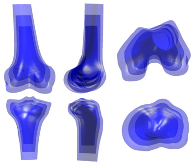
A MATLAB (MathWorks, Natick, MA) script is provided to facilitate visualization of the anatomy and SSMs (filename: SSMvisualization.m). It imports Registers.mat (described under ‘Registers’ in the Data Records section) and, after the user selects either the femur or tibia, constructs a statistical shape model using PCA. The code enables visualization of the modes of shape variation through two-dimensional overlays at ±2 standard deviations in multiple views, animated videos illustrating each mode in multiple views, and scatter plots of principal component scores for all subjects grouped by sex and race or ethnicity. All outputs are automatically saved in their appropriate formats to a folder labeled ‘outputs’.

This framework is intended to demonstrate how to interact with and visualize the statistical shape models and their instances. It is not intended to provide an exhaustive set of analysis or visualization tools, and users are encouraged to adapt and extend the framework to suit their own applications.

Contributing New and Updated Geometries

New geometries can be added to the dataset by contacting the authors ([email protected] and [email protected]). The authors will check new or revised content for accuracy and completeness and update the folders with credit of the contributors highlighted on this website.

Additional Contributors

Jenelys Cox, The University of Denver

License

Data available for download is governed by the Creative Commons Attribution-NonCommercial license: CC BY-NC 4.0

Please note the original NMDID data is governed by the license terms described here: https://nmdid.unm.edu/resources/data-use

Liability Agreement

The Data is provided “as is” with no express or implied warranty or guarantee. The University of Denver and the Center for Orthopaedic Biomechanics do not accept any liability or provide any guarantee in connection with uses of the Data, including but not limited to, fitness for a particular purpose and noninfringement. The University of Denver and the Center for Orthopaedic Biomechanics are not liable for direct or indirect losses or damage, of any kind, which may arise through the use of this data.

Citations

This work has been submitted and is in review at the following journal:
Kindy, G., Alsaadi, O., Laz, P.J. “Anatomical Variation in the Knee: A Dataset of 3D Bone Models and Statistical Shape Models.” Nature: Scientific Data, in review.

DOI for this page: https://doi.org/10.56902/COB.av.2026.0
References

1. Edgar, H. et al. New Mexico Decedent Image Database (NMDID). https://doi.org/10.25827/5S8C-N515 (2020) doi:10.25827/5S8C-N515.
2. Barton, B. et al. 2023 National Healthcare Quality and Disparities Report.
3. Fugit, W. J., Aram, L. J., Bayoglu, R. & Laz, P. J. Accuracy tradeoffs between individual bone and joint-level statistical shape models of knee morphology. Med. Eng. Phys. 130, 104203 (2024).
4. Kroon, D.-J. Finite Iterative Closest Point. (2024).
5. Myronenko, A. & Xubo Song. Point Set Registration: Coherent Point Drift. IEEE Trans. Pattern Anal. Mach. Intell. 32, 2262–2275 (2010).
6. ANSYS. Meshing User’s Guide. (2024).
7. Mahfouz, M., Abdel Fatah, E. E., Bowers, L. S. & Scuderi, G. Three-dimensional Morphology of the Knee Reveals Ethnic Differences. Clin. Orthop. 470, 172–185 (2012).
8. Ma, Q.-L. et al. A Comparison Between Chinese and Caucasian 3-Dimensional Bony Morphometry in Presimulated and Postsimulated Osteotomy for Total Knee Arthroplasty. J. Arthroplasty 32, 2878–2886 (2017).
9. Wang, S. W., Feng, C. H. & Lu, H. S. A study of Chinese knee joint geometry for prosthesis design. Chin. Med. J. (Engl.) 105, 227–233 (1992).
10. Van Oevelen, A. et al. Personalized statistical modeling of soft tissue structures in the knee. Front. Bioeng. Biotechnol. 11, 1055860 (2023).
11. Audenaert, E. A. et al. Statistical Shape Modeling of Skeletal Anatomy for Sex Discrimination: Their Training Size, Sexual Dimorphism, and Asymmetry. Front. Bioeng. Biotechnol. 7, 302 (2019).